Profiling
This tutorial describes how to use OpenMDAO’s simple instance based profiling capability. Python has several good profilers available for general python code, but the advantage of OpenMDAO’s simple profiler is that it limits the functions of interest down to a relatively small number of important OpenMDAO functions, which helps prevent information overload. Also, the OpenMDAO profiler lets you view the profiled functions grouped by the specific problem, system, group, driver, or solver that called them. This provides insight into which parts of your model are more expensive, even when different parts of your model use many of the same underlying functions.
To use profiling, you first have to call profile.setup. This must happen after your system tree has been defined. This is necessary because the setup process traverses down the tree searching for instance methods to wrap with profiling information, and if those instance methods don’t exist yet then they cannot be wrapped. You must pass a top level object, typically your Problem object, to profile.setup.
After profiling has been set up, you then call profile.start to start collection of profiling data. If for some reason you want to only collect profiling data during a particular part of execution, you can call profile.stop to turn off collection. For example:
from openmdao.api import Problem, Group
from openmdao.api import profile

prob = Problem(root=Group())

# define my model...

profile.setup(prob)
profile.start()

prob.setup()

prob.run()

profile.stop()

# do some other stuff that I don't want to profile...
There are a few advanced options to profile.setup, but in general you won’t need them. Consult the docstring to learn more.
After your script is finished running, you should have two new files, prof_raw.0 and funcs_prof_raw.0 in your current directory. If you happen to have activated profiling for an MPI run, then you’ll have a copy of those two files for each MPI process, so prof_raw.0, prof_raw.1, etc.
There are two command scripts you can run on those raw data files. The first is proftotals. Running that on raw profiling files will give you CSV formatted output containing total runtime and total number of calls for each profiled function. For example: proftotals prof_raw.* might give you output like the following:
Function Name, Total Time, Calls
.calc_gradient.2, 40.9992446899, 1
.calc_gradient.0, 40.9991188049, 1
.calc_gradient.1, 40.9931678772, 1
.LinearGaussSeidel.solve.2, 30.7603917122, 31
.LinearGaussSeidel.solve.1, 29.2816333771, 31
.LinearGaussSeidel.solve.0, 29.000962019, 31
._transfer_data.2, 20.4067265987, 352
._transfer_data.0, 15.5122716427, 352
._transfer_data.1, 13.8179996014, 352
...
The second command script is profview. By default, it generates an html file called profile_icicle.html that uses a d3-based icicle plot to show the function call tree. The file should be viewable in any browser. Hovering over a box in the plot will show the function pathname, the local and total elapsed time for that function, and the local and total number of calls for that function. Clicking on a box will collapse the view so that that box’s function will become the top box and only functions called by that function will be visible. The top box before any box has been collapsed does not represent a real function. Instead, it shows the sum of the elapsed times of all of the top level functions as its local time, and the total time that profiling was active as its total time. If the total time is greater than the local time, that indicates that some amount of time was taken up by functions that were not being profiled.
The profiling data needed for the viewer is included directly in the html file, so the file can be passed around and viewed by other people. It does however require network access in order to load the d3 library.
To pop up the viewer in a browser immediately, use the –show option, for example:
profview raw_prof.* --show
You should then see something like this:
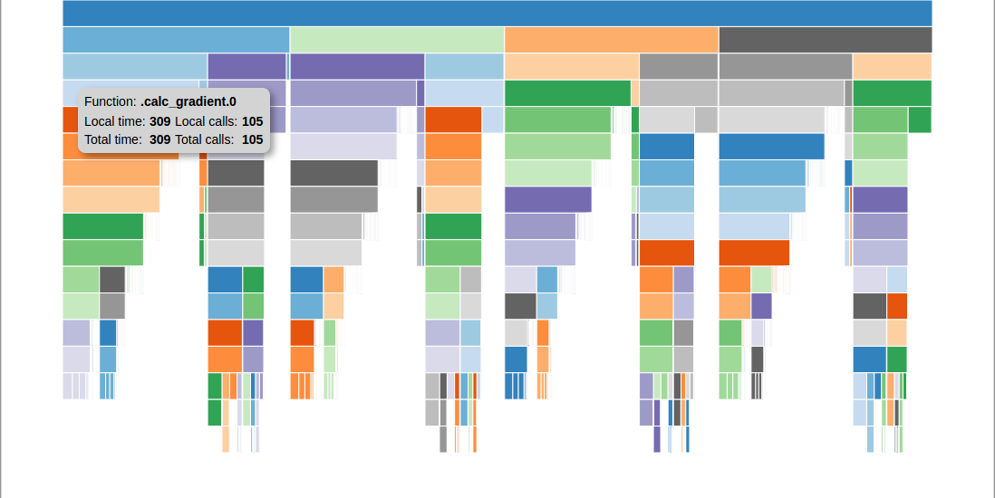
An example of a profile icicle viewer.
If you use the -v sunburst option to profview, you will instead see a sunburst plot of the profile data. It functions similarly to the icicle viewer except that the functions are laid out radially instead of linearly. A sunburst viewer looks like this:

An example of a profile sunburst viewer.