The Sellar Problem
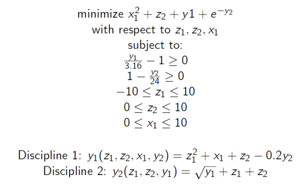
This tutorial illustrates how to set up a coupled disciplinary problem in OpenMDAO and prepare it for optimization, using the Sellar Problem consisting of two disciplines as follows:
| [SELLAR] | Sellar, R. S., Batill, S. M., and Renaud, J. E., “Response Surface Based, |
Variables z1, z2, and x1 are the design variables. Both disciplines are functions of z1 and z2, so they are called the global design variables, while only the first discipline is a function of x1, so it is called the local design variable. The two disciplines are coupled by the coupling variables y1 and y2. Discipline 1 takes y2 as an input, and computes y1 as an output, while Discipline 2 takes y1 as an input and computes y2 as an output. This coupling creates a non-linear system of equations which must be satisfied for valid solutions.
First, disciplines 1 and 2 were implemented in OpenMDAO as components.
# For printing, use this import if you are running Python 2.x
from __future__ import print_function


import numpy as np

from openmdao.core.component import Component


class SellarDis1(Component):
    """Component containing Discipline 1."""

    def __init__(self):
        super(SellarDis1, self).__init__()

        # Global Design Variable
        self.add_param('z', val=np.zeros(2))

        # Local Design Variable
        self.add_param('x', val=0.)

        # Coupling parameter
        self.add_param('y2', val=1.0)

        # Coupling output
        self.add_output('y1', val=1.0)

    def solve_nonlinear(self, params, unknowns, resids):
        """Evaluates the equation
        y1 = z1**2 + z2 + x1 - 0.2*y2"""

        z1 = params['z'][0]
        z2 = params['z'][1]
        x1 = params['x']
        y2 = params['y2']

        unknowns['y1'] = z1**2 + z2 + x1 - 0.2*y2

    def jacobian(self, params, unknowns, resids):
        """ Jacobian for Sellar discipline 1."""
        J = {}

        J['y1','y2'] = -0.2
        J['y1','z'] = np.array([[2*params['z'][0], 1.0]])
        J['y1','x'] = 1.0

        return J


class SellarDis2(Component):
    """Component containing Discipline 2."""

    def __init__(self):
        super(SellarDis2, self).__init__()

        # Global Design Variable
        self.add_param('z', val=np.zeros(2))

        # Coupling parameter
        self.add_param('y1', val=1.0)

        # Coupling output
        self.add_output('y2', val=1.0)

    def solve_nonlinear(self, params, unknowns, resids):
        """Evaluates the equation
        y2 = y1**(.5) + z1 + z2"""

        z1 = params['z'][0]
        z2 = params['z'][1]
        y1 = params['y1']

        # Note: this may cause some issues. However, y1 is constrained to be
        # above 3.16, so lets just let it converge, and the optimizer will
        # throw it out
        y1 = abs(y1)

        unknowns['y2'] = y1**.5 + z1 + z2

    def jacobian(self, params, unknowns, resids):
        """ Jacobian for Sellar discipline 2."""
        J = {}

        J['y2', 'y1'] = .5*params['y1']**-.5
        J['y2', 'z'] = np.array([[1.0, 1.0]])

        return J
For the most part, construction of these Components builds on what you learned in previous tutorials. In building these disciplines, we gave default values to all of the params and unknowns so that OpenMDAO can allocate the correct size in the vectors. The global design variables z1 and z1 were combined into a 2-element ndarray.
Note
Discipline2 contains a square root of variable y1 in its calculation. For negative values
of y1, the result would be imaginary, so the absolute value is taken before the square root
is applied. This component is clearly not valid for y1 < 0, but some solvers could
occasionally force y1 to go slightly negative while trying to converge the two disciplines . The inclusion
of the absolute value solves the problem without impacting the final converged solution.
We have written two (very simple) analysis components. If you were working on a real problem, these would your components could be more complex, or could potentially be wrappers for external analysis components. But keep in mind that from an optimization point of view, whether they are simple tools or wrappers for real analyses, OpenMDAO still views them as components with params, unknowns, resids and a solve_nonlinear function, and optionally a jacobian function.
At this point we’ve written the components, but we haven’t combined them together into any kind of model. That’s what we’ll get to next!
Building the Sellar Model
Next we will set up the Sellar Problem and optimize it. First we will take the Components that we just created and assemble them into a Group. We will also add the objective and the multivariable constraints to the problem using a utility Component that can be used when you have simple equations for things like objectives and constraints.
from openmdao.components.execcomp import ExecComp
from openmdao.components.paramcomp import ParamComp
from openmdao.core.group import Group
from openmdao.solvers.nl_gauss_seidel import NLGaussSeidel

class SellarDerivatives(Group):
    """ Group containing the Sellar MDA. This version uses the disciplines
    with derivatives."""

    def __init__(self):
        super(SellarDerivatives, self).__init__()

        self.add('px', ParamComp('x', 1.0), promotes=['*'])
        self.add('pz', ParamComp('z', np.array([5.0, 2.0])), promotes=['*'])

        self.add('d1', SellarDis1(), promotes=['*'])
        self.add('d2', SellarDis2(), promotes=['*'])

        self.add('obj_cmp', ExecComp('obj = x**2 + z[1] + y1 + exp(-y2)',
                                     z=np.array([0.0, 0.0]), x=0.0, y1=0.0, y2=0.0),
                 promotes=['*'])

        self.add('con_cmp1', ExecComp('con1 = 3.16 - y1'), promotes=['*'])
        self.add('con_cmp2', ExecComp('con2 = y2 - 24.0'), promotes=['*'])

        self.nl_solver = NLGaussSeidel()
        self.nl_solver.options['atol'] = 1.0e-12
We use add to add Components or Systems to a Group. The order you add them to your Group is the order they will execute, so it to add them in the correct order. Here, this means starting with the ParamComps, then adding our disciplines, and finishing with the objective and constraints.
We have also decided to declare all of our connections to be implicit by using the promotes argument when we added any component. When you promote ‘*’, that means that every param and unknown is available in the parent system. Thus, if you wanted to connect something to variable y1, you would address it with the string y1 instead of dis1.y1. The following is also valid
self.add('d1', SellarDis1(), promotes=['x', 'z', 'y1', 'y2'])
In this case, our two disciplines both promote y1 and y2. Discipline 1 provides y1 as a source and discipline 2 needs it as a param, so when both of them promote y1, the connection is made for you, implicitly.
Due to the implicit connections, we now have a cycle between the two disciplines. This is fine because a nonlinear solver can converge the cycle to arrive at values of y1 and y2 that satisfy the equations in both disciplines. We have selected the NLGaussSeidel solver (i.e., fixed point iteration), which will converge the model in our Group. We also specify a tighter tolerance in the solver’s options dictionary, overriding the 1e-6 default.
The objective and constraints are defined with the ExecComp, which is really a shortcut for creating a Component that is a simple function of other variables in the model. ExecComp is just there as a convenience for users. You don’t have to use it, if for example you wrote your own component that already outputs objective and constraint variables.
self.add('obj_cmp', ExecComp('obj = x**2 + z[1] + y1 + exp(-y2)',
                             z=np.array([0.0, 0.0]), x=0.0, y1=0.0, y2=0.0),
         promotes=['*'])
This creates a component named ‘obj_comp’ with inputs ‘x’, ‘z’, ‘y1’, and ‘y2’, and with output ‘obj’. The first argument is a string expression that contains the function. OpenMDAO can parse this expression so that the solve_nonlinear and jacobian methods are taken care of for you. Notice that standard math functions like exp are available to use. Because we promote every variable in our call to add, all of the inputs variables are automatically connected to sources in the model. We also specify our default initial values as the remaining arguments for the ExecComp. You are not required to do this for scalars, but you must always allocate the array inputs (‘z’ in this case). The output of the objective equation is stored in the promoted output ‘obj’.
So that’s three ExecComp instances, one each for the objective and two constraints. Now, that we are done creating the Group for the Sellar problem, let’s hook it up to an optimizer.
Setting up the Optimization Problem
Any analysis or optimization in OpenMDAO always happens in a Problem instance, with a Group at the root. Here we set our Sellar group as root. Then we set the driver to be the ScipyOptimizer, which wraps scipy’s minimize function.
Note
Scipy offers a number of different optimizers, but COBYLA and SLSQP are the only two choices that support constrained optimization. SLSQP is the only gradient based method of the two. If you want a broader selection of optimizers, you can install the pyopt_sparse library, which we also have a wrapper for.
from openmdao.core.problem import Problem
from openmdao.drivers.scipy_optimizer import ScipyOptimizer

top = Problem()
top.root = SellarDerivatives()

top.driver = ScipyOptimizer()
top.driver.options['optimizer'] = 'SLSQP'
top.driver.options['tol'] = 1.0e-8

top.driver.add_param('z', low=np.array([-10.0, 0.0]),
                     high=np.array([10.0, 10.0]))
top.driver.add_param('x', low=0.0, high=10.0)

top.driver.add_objective('obj')
top.driver.add_constraint('con1')
top.driver.add_constraint('con2')

top.setup()
top.run()

print("\n")
print( "Minimum found at (%f, %f, %f)" % (top['z'][0], \
                                         top['z'][1], \
                                         top['x']))
print("Coupling vars: %f, %f" % (top['y1'], top['y2']))
print("Minimum objective: ", top['obj'])
Next we add the parameter for ‘z’. Recall that the first argument for add_param is a string containing the name of a variable declared in a ParamComp. Since we are promoting the output of this pcomp, we use the promoted name, which is ‘z’ (and likewise we use ‘x’ for the other parameter.) Variable ‘z’ is an 2-element array, and each element has a different set of bounds defined in the problem, so we specify the low and high attributes as numpy arrays. If you are ok with the same low or high for all elements of your design variable array, you could also give a scalar for those arguments.
Next, we add the objective by calling add_objective on the driver giving it the promoted path of the quantity we wish to minimize. All optimizers in OpenMDAO try to minimize the value of the objective, so to maximize a variable, you will have to place a minus sign in the expression you give to the objective ExecComp.
Finally we add the constraints using the add_constraint method, which takes any valid unknown in the model as the first argument. Constraints in OpenMDAO are defined so that a negative value means the constraint is satisfied, and a positive value means it is violated. When a constraint is equal to zero, it is called an ‘active’ constraint.
Don’t forget to call setup on your Problem before calling run. Also, we are using the Python 3.x print function to print results. To keep compatibility with both Python 2.x and 3.x, don’t forget the following import at the top of your python file:
from __future__ import print_function
If we take all of the code we have written in this tutorial and place it into a file called sellar_MDF_optimization.py and run it, the final output will look something like:
$ python sellar_MDF_optimization.py
.
.
.
Minimum found at (1.977639, ...0.000000, ...0.000000)
Coupling vars: 3.160000, 3.755278
Minimum objective:  3.18339395045
Depending on print settings, there may be some additional optimizer output where the ellipses are. This is the expected minimum for the Sellar problem.
Sellar with an Implicit Component
We have just built an implementation of the Sellar problem where the two disciplines are connected with a cycle. We could also sever the direct connection and close the gap with an implicit component. The purpose of this component is to express as a residual the difference between the output side and the input side of the connection that we are replacing.
In Sellar, we will leave the y1 connection and replace the y2 connection. First we need to write the component to replace the connection:
class StateConnection(Component):
    """ Define connection with an explicit equation"""

    def __init__(self):
        super(StateConnection, self).__init__()

        # Inputs
        self.add_param('y2_actual', 1.0)

        # States
        self.add_state('y2_command', val=1.0)

    def apply_nonlinear(self, params, unknowns, resids):
        """ Don't solve; just calculate the residual."""

        y2_actual = params['y2_actual']
        y2_command = unknowns['y2_command']

        resids['y2_command'] = y2_actual - y2_command

    def solve_nonlinear(self, params, unknowns, resids):
        """ This is a dummy comp that doesn't modify its state."""
        pass

    def jacobian(self, params, unknowns, resids):
        """Analytical derivatives."""

        J = {}

        # State equation
        J[('y2_command', 'y2_command')] = -1.0
        J[('y2_command', 'y2_actual')] = 1.0

        return J
So this Component has one state and one param. The StateConnection component will bridge the gap between the output of y2 from Discipline2 and the input for y2 in Discipline1. The solver sets the new value of y2 based on the models residuals, which now include the difference between ‘y2’ leaving Discipline2 and the ‘y2’ entering Discipline1. So the solve_nonlinear method does nothing, but we need to define apply_nonlinear to return this residual. Residuals live in the resids vector, so we set:
resids['y2_command'] = y2_actual - y2_command
We also define the Jacobian method, and the derivatives are trivial to compute.
Next, we need to modify the model that we defined in SellarDerivatives to break the connection and use the StateConnection component.
from openmdao.solvers.newton import Newton

class SellarStateConnection(Group):
    """ Group containing the Sellar MDA. This version uses the disciplines
    with derivatives."""

    def __init__(self):
        super(SellarStateConnection, self).__init__()

        self.add('px', ParamComp('x', 1.0), promotes=['*'])
        self.add('pz', ParamComp('z', np.array([5.0, 2.0])), promotes=['*'])

        self.add('state_eq', StateConnection())
        self.add('d1', SellarDis1(), promotes=['x', 'z', 'y1'])
        self.add('d2', SellarDis2(), promotes=['z', 'y1'])
        self.connect('state_eq.y2_command', 'd1.y2')
        self.connect('d2.y2', 'state_eq.y2_actual')

        self.add('obj_cmp', ExecComp('obj = x**2 + z[1] + y1 + exp(-y2)',
                                     z=np.array([0.0, 0.0]), x=0.0, y1=0.0, y2=0.0),
                  promotes=['x', 'z', 'y1', 'obj'])
        self.connect('d2.y2', 'obj_cmp.y2')

        self.add('con_cmp1', ExecComp('con1 = 3.16 - y1'), promotes=['*'])
        self.add('con_cmp2', ExecComp('con2 = y2 - 24.0'), promotes=['con2'])
        self.connect('d2.y2', 'con_cmp2.y2')

        self.nl_solver = Newton()
The first thing to notice is that we no longer promote the variable y2 up to the group level. We need to add the connections manually because we really have two different variables: ‘d1.y2’ and ‘d2.y2’. In addition to the two connections to the ‘state_eq’ component, we also need to manually connect y2 to the objective and one of the constraints.
We have also switched the solver to the Newton solver, since we no longer are iterating around a loop. Don’t forget to change your import. The default settings should be fine for Sellar.
Otherwise, there are no other differences in the model, and the remaining optimization set up is the same as before. However, a small change in printing our results is required because ‘y2’ no longer exists in the group. We must print either ‘state_eq.y2_command’ or ‘d2.y2’ instead. It doesn’t matter which one, since they should only differ by the solver tolerance at most.
from openmdao.core.problem import Problem
from openmdao.drivers.scipy_optimizer import ScipyOptimizer

top = Problem()
top.root = SellarStateConnection()

top.driver = ScipyOptimizer()
top.driver.options['optimizer'] = 'SLSQP'
top.driver.options['tol'] = 1.0e-8

top.driver.add_param('z', low=np.array([-10.0, 0.0]),
                     high=np.array([10.0, 10.0]))
top.driver.add_param('x', low=0.0, high=10.0)

top.driver.add_objective('obj')
top.driver.add_constraint('con1')
top.driver.add_constraint('con2')

top.setup()
top.run()

print("\n")
print( "Minimum found at (%f, %f, %f)" % (top['z'][0], \
                                         top['z'][1], \
                                         top['x']))
print("Coupling vars: %f, %f" % (top['y1'], top['d2.y2']))
print("Minimum objective: ", top['obj'])
You can verify that the new model arrives at the same optimum as the old one.